This is an old revision of the document!
Table of Contents
Intro
NSW Spatial Services have undertaken a program to map all of NSW using lidar (light detecting and ranging) For details, see information on their elevation program.
Elevation data can best be accessed through the Geoscience Australia ELVIS program.
It can then processed with a GIS such as QGIS to create useful topographic maps. Instructions below are specifically for use with QGIS, though the general outline may be useful for other GISs.
Resources
Managing DEMs
Downloading data
While data can be downloaded in an ad hoc manner, if you are regularly processing DEMs, it is better to have the DEM tiles already downloaded. Download tiles by 1:100k map area, which is 0.5 x 0.5 degree squares. Each 1:100k map area ranges from around 2GB to 6GB of data, depending on the number of 2m DEMs vs 1m DEMs, and other factors.
The Sydney basin and Blue Mountains is around 50GB all up.
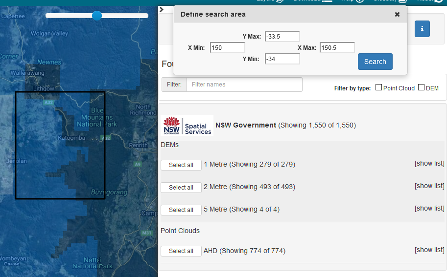
For example, to request data for the Katoomba 1:100k map area (-33.5,150,-34,150.5), see the screenshot below, and Select All DEMs:
Below are the 1:100k map areas around Sydney:
| 8833_gulgong | 8933_merriwa | 9033_muswellbrook | 9133_camberwell | 9233_dungog | 9333_buladelah | 9433_forster |
| 8832_mudgee | 8932_mt_pomany | 9032_howes_valley | 9132_cessnock | 9232_newcastle | 9332_port_stephens | |
| 8831_bathurst | 8931_wallerawang | 9031_st_albans | 9131_gosford | 9231_lake_macquarie | ||
| 8830_oberon | 8930_katoomba | 9030_penrith | 9130_sydney | |||
| 8829_taralga | 8929_burragorang | 9029_wollongong | 9129_port_hacking | |||
| 8828_goulburn | 8928_moss_vale | 9028_kiama | ||||
| 8827_braidwood | 8927_ulladulla | 9027_jervis_bay |
Pre-processing data
The following may be useful for Windows users.
Below is a Windows Powershell script that will
- move any old DEMs and DEMs from a different zone (you can't mix zones in a virtual raster) to an archive sub-folder
- extract the raw data from the remaining zip files
- convert all of the .ASC files to GeoTIFF
- move the old zip files to a current sub-folder
- zip the current and archive sub-folders to temp.zip
- create a virtual raster (.vrt) file of all of the GeoTiffs
You will need to replace the Environment variables with your own - lines starting with $Env.
Usage is: buildvrt.ps1 <zipFile> <targetFolder> eg buildvrt.ps1 <zipFile> <targetFolder>
- buildvrt.ps1
$zipFile=$args[0]
$targetFolder=$args[1]

# Unzip files from all subdirectories to new folder
Expand-Archive -LiteralPath $zipFile -DestinationPath $targetFolder
Get-ChildItem -Path "$targetFolder\*.zip" -Recurse | Move-Item -Destination $targetFolder
Get-ChildItem -Path $targetFolder -Directory | Remove-Item -Recurse

# Create hash of zip files, by name (location, date)
$zipFileList = @{}
Get-ChildItem -Path "$targetFolder\*.zip" -Name | ForEach-Object {
	$zipFileList.add($_, @{})
	$_ -match '(\d{7})_(\d{2})'
	$zipFileList[$_]['location'] = $Matches.1
	$zipFileList[$_]['zone'] = $Matches.2
	$_ -match '[^_\d](\d{6})'
	$zipFileList[$_]['date'] = $Matches.1
}
# $zipFileList | ConvertTo-Json

# Create hash of location (date, name)
$locationList = @{}
$zoneCount = @{}
$zipFileList.keys | ForEach-Object {
	if($locationList[$zipFileList[$_]['location']]) {
		$t = $locationList[$zipFileList[$_]['location']]
		$t.add($zipFileList[$_]['date'],$_)
	} else {
		$t = @{}
		$t.add($zipFileList[$_]['date'],$_)
		$locationList.add($zipFileList[$_]['location'],$t)
	}
	if($zoneCount[$zipFileList[$_]['zone']]) {
		$zoneCount[$zipFileList[$_]['zone']]++
	} else {
		$zoneCount[$zipFileList[$_]['zone']] = 1
	}
}
# $locationList | ConvertTo-Json
# $zoneCount | ConvertTo-Json

# Create archive folder
$archiveFolder = "$targetFolder\archive"
If(!(test-path $archiveFolder))
{
      New-Item -ItemType Directory -Force -Path $archiveFolder
}

# Sort each location by date desc, and move old files to /archive
$locationList.keys | ForEach-Object {
	$i=0
	$locationList[$_].GetEnumerator() | sort key -des | ForEach-Object {
		if ($i -eq 0) {
			$i++
			return}
		else {
			#$_ | ConvertTo-Json
			$s = $_.Value
			Move-Item -Path "$targetFolder\$s" -Destination "$targetFolder\archive\$s"
		}
	}
}

# You can't build a VRT with files from a different projection, so
# delete files from outside main zone
# This could probably be altered to include a step to reproject those files
$mainZone = ''
$zoneCount.GetEnumerator() | sort value -des | select -first 1 | ForEach-Object {
	$mainZone = $_.Name
}

$zipFileList.keys | ForEach-Object {
	if($zipFileList[$_]['zone'] -ne $mainZone) {
		Remove-Item -Path "$targetFolder\$_"
	}
}

Get-ChildItem -Path "$targetFolder\*.zip" | Expand-Archive -DestinationPath $targetFolder
$Env:Path += ";C:\OSGEO4~1\apps\Python27\Scripts;C:\OSGEO4~1\bin"
$Env:GDAL_DATA="C:\OSGEO4~1\share\gdal"
$Env:GDAL_DRIVER_PATH="C:\OSGEO4~1\bin\gdalplugins"
$Env:PROJ_LIB="C:\OSGEO4~1\share\proj"

Get-ChildItem -Path "$targetFolder\*.asc" | ForEach-Object {
	$srcFile = $_.FullName
	$destFile = $_.FullName -replace '.asc', '.tif'
	&"gdal_translate.exe" -of "GTiff" $srcFile $destFile
}

Get-ChildItem -Path "$targetFolder\*.asc" | Remove-Item -Recurse
Get-ChildItem -Path "$targetFolder\*.html" | Remove-Item -Recurse
Get-ChildItem -Path "$targetFolder\*.prj" | Remove-Item -Recurse
Get-ChildItem -Path "$targetFolder\*.xml" | Remove-Item -Recurse

# Create current folder
$currentFolder = "$targetFolder\current"
If(!(test-path $currentFolder))
{
      New-Item -ItemType Directory -Force -Path $currentFolder
}

# Move zip files to current folder
Move-Item -Path "$targetFolder\*.zip" -Destination "$currentFolder"

# Zip /archive & /current to new zip folder
Compress-Archive -Path "$targetFolder\current", "$targetFolder\archive" -DestinationPath "$targetFolder\temp.zip"

# Create 2m vrt
New-Item "$targetFolder\input.txt"
Get-ChildItem -Path "$targetFolder\*.tif" | Add-Content "$targetFolder\input.txt"
&"gdalbuildvrt.exe" -resolution lowest -input_file_list "$targetFolder\input.txt" "$targetFolder\temp.vrt"
It is possible to then build a larger virtual raster from the individual 1:100k virtual rasters.
Loading data
Loading up a large virtual raster into QGIS can be very slow, as can manipulating it. However, you can quickly load up a smaller section of the map using the following steps:
- create a polygon using https://maps.ozultimate.com/
- download the polygon using the Export drawn data to GeoJSON function
- load up the Python console (Plugins→Python Console or Ctrl+Alt+P on Windows)
- run the following command (replace file locations with your own)
resultClip = processing.runAndLoadResults("gdal:cliprasterbymasklayer", { 'ALPHA_BAND' : False, 'CROP_TO_CUTLINE' : True, 'DATA_TYPE' : 0, 'EXTRA' : '', 'INPUT' : 'E:/geodata/8930_katoomba/area.vrt', 'KEEP_RESOLUTION' : False, 'MASK' : 'C:/Users/Downloads/data.geojson', 'MULTITHREADING' : False, 'NODATA' : None, 'OPTIONS' : '', 'OUTPUT' : 'TEMPORARY_OUTPUT', 'SET_RESOLUTION' : False, 'SOURCE_CRS' : None, 'TARGET_CRS' : None, 'X_RESOLUTION' : None, 'Y_RESOLUTION' : None })
Topographic maps
There are several primary data items for topographic maps that can be generated using the DEM data from the NSW Lidar. The main ones are:
- Contours
- Hydrology (Stream Network)
- Clifflines
The steps below are works in progress to determine effective (the best?) ways to extract the various items out of the DEM data for use in topographic maps. Any feedback/suggestions of improvements are welcome.
Merge DEMs
The NSW DEM data is supplied in 2km squares. The squares need to be merged into a single DEM for further operations.
Most of the eastern ranges, where a lot of bushwalking happens, are 2m DEMs. The coast is typically 1m, and the western slopes and plains are 5m (with major rivers 1m!). Be careful if you need to merge DEMs with different resolutions - see below for more details.
Virtual Raster
While merging can be done in theory using a Virtual Raster (Raster- > Miscellaneous → Build Virtual Raster… ), I have had poor performance with this (including recent version 3.12 Bucuresti). Any operation seems to result in screen redrawing, so moving around and zooming in and out is slow and painful.
That said, if you are just using the Virtual Raster for future steps, then the limitations from the screen redrawing may not be important.
QGIS uses gdalbuildvrt. Uncheck “Place each input file into a separate band”, and if you are using files with different resolutions (eg 1m and 2m), change the Resolution to Highest or Lowest as appropriate. You can also change the Resolution to User, and set the optional -tr switch (eg -tr 1 1 or -tr 2 2)
Merge Raster
I generally use the the Raster- > Miscellaneous → Merge… function
QGIS uses gdal_merge, which defaults to using the resolution of the first file. This is not always desired. It can be controlled by using the optional -ps (pixel size) switch. For example, if you have a combination of 1m and 2m DEMs, you can use -ps 1 1 to force them to a merged 1m DEM, or -ps 2 2 to force them to merge to a 2m DEM.
Fill Sinks
From the initial DEM, first step is to Fill Sinks. Otherwise you will get sinks in the middle of watercourses, which will impact contours and stream networks. Note that the this approach needs to be used with care in areas where there are actual depressions.
There are various related tools in the Processing Toolbox that will do this, including:
- SAGA : Terrain Analysis - Hydrology : Fill Sinks
- SAGA : Terrain Analysis - Hydrology : Fill Sinks (Wang and Liu)
- SAGA : Terrain Analysis - Hydrology : Fill Sinks XXL (Wang and Liu)
The results from all will be similar, but the Wang and Liu versions should be faster.
There are other approaches that deepen channels rather than fill sinks in order to get a hydrologically sound drainage network. For example
- SAGA : Terrain Analysis - Hydrology : Sink Removal
has an option for this.
Contours
Basic Processing
There are various contour extraction algorithms in QGIS, for example:
- GDAL : Raster Extraction : Contour (same as Raster → Extraction → Contour…)
Below is an example of contours created without and with sink removal. The contours on the right have been derived from a DEM where the sinks (in yellow on the left) have been filled.


Even with sink removal, small
Simplifying
Vectors can be compressed by using something like:
- Vector geometry : Simplify
A tolerance of 1(m) seems reasonable for 1:25000 mapping. Smaller tolerances may be appropriate for larger scale maps (eg 1:10000, 1:5000).
For more options in compression, look at:
- GRASS : v.generalize
V.generalize can also be used to smooth contours - possibly best done prior to simplificiation
Cleaning
Once simplified, it is worth removing small closed loops, such as those in the image below.

Here is one approach, which involves adding a length attribute to each contour, and removing those that fall below a certain length. It may cause issues if you have short sections of contour near the edge of the map that you need.
- Open Attribute Table (F6)
- Open field calculator (Ctrl+I)
- Add new attribute length, calculated as $length

- Select all features and filter on length < 25 (or whatever length is appropriate for your scale)

Contour Labelling
See separate page on QGIS Contour Labelling
Hydrology (Stream Network)
The starting point for hydrology is a hydrologically sound DEM, as above. Use a fill sinks or channel deepening algorithm.
Catchment Areas
Next step is to create Catchment Areas. Again, there is a Catchment Area tool (in fact several), and six methods within the tool. For the purpose of delineating watercourses in steep terrain, the choice of method probably makes little difference.
- SAGA : Terrain Analysis - Hydrology : Catchment Area
This gives an output that is best viewed in log scale. You can do this via
- Raster → Raster Calculator…
- log10 ( “Filled DEM@1” )
Use the log scale version to determine the cutoff for what streams you want to see and which ones are too small. 10000 seems to give comparable results to the existing 1:25000 maps.
Note that if you don't have the entirety of the catchment, you may get erroneous results.
Channel Network
The following tool can be used to create channels (streams) - there are other options:
- SAGA : Terrain Analysis - Channels : Channel Network
Use
- Elevation = Filled DEM
- Initiation Grid = Catchment Area
- Initiation Type = Greater Than
- Initiation Threshold = 10000 (or whatever number you have determined)

Classification
For 1:25000 maps, I've had reasonable results from using the following formula in the Raster Calculator to classify the streams into categories. Different scales may need different bounds, and this doesn't account for significantly larger rivers.
( log10 ( “Catchment Area@1” ) >= x) * ( log10 ( “Catchment Area@1” ) < y) * (“Channel Network@1” != 0)
- Intermittent: 4-6.15 (x-y)
- Minor: 6.15-7.4
- Major: 7.4+
Convert to Vector and Simplify
Convert to vector using r.to.vect

The raw stream data is very jagged. Smooth using
- v.generalize
- Algorithm = Hermite (there are other options which can be used, but Hermite has the smoothed line passing through the points of the original)
- Maximal tolerance value = 20 (in m, obviously scale dependent)
Simplify using using:
- Vector geometry : Simplify
Tolerance:?
Clifflines
The steps below are being developed for use in the Blue Mountains, a region that has a significant number of relatively vertical sandstone cliffs. It may be less effective in different terrain.
This is more a set of ideas than a fully fledged process. The main aims are to get a set of steps that can largely be automated, and that create cliffline vectors that are running in the correct direction. There is still some way to go on this!
Initial analysis of slope, aspect
SAGA → Terrain Analysis - Morphometry → Slope, Aspect, Curvature
Extract
Slope, Aspect
using DEM and [1] Maximum Triangle Slope (Tarboton (1997)). I haven't tested any other algorithms.
Cliff areas can be identified using a range of say 60-90 and 70-90 degrees on the Slope file. Using 60-90 degrees helps connect logical cliffs and avoid small breaks.
Initial Cleaning
Next convert data to 1 bit (1,2 not 0,1, as Sieve ignores 0s) using Raster Calculator. Formula is: (Slope > 60) + 1
Then Sieve resulting data using a Threshold of 100 and 8-connectedness to get rid of small non-connected cliffs. Note above that Sieve doesn't like 0s.
Also good to rerun Sieve with smaller Threshold (1-10) and 4-connectedness to a) get rid of some small dangles. b) fill small holes.
Additional smoothing can be done using a User Defined Filter with the following matrix. This will apply some smoothing by allowing you to reclassify the pixel values, and remove single pixel indentations like this:
000    000
101 -> 111
111    111
and single pixel protrusions like this:
000    000
010 -> 000
111    111
The main problem is that the matrix has to be defined each time in QGIS. There doesn't seem to be an option to load it. Possibly this can be done outside QGIS.
Matrix is:
0.0 0.5 0.0
0.5 0.5 0.5
0.0 0.5 0.0
If the original matrix is 0/1 then the cutoff will be 1.5
If the original matrix is 1/2 then the cutoff will be 3.5
This step could be run multiple times - some testing would need to be done to determine how many times.
Other options for cleaning the data include a plugin called LecoS, but this doesn't work on QGIS 3. Another possibility is Shrink and Expand - radius 1? But this also creates some new holes that didn't previously exist, so not ideal.
Thinning
Convert back to 0/1 data using Raster Calculator
Use Translate: set Output Data Type = Byte, set NoData = 0
Run r.thin - r.thin is quite picky about the input file format. Needs to be NULL/non-NULL (not float or int). The Translate process above provides this. The previous two steps could be combined into one. Also, this file may need to be explicitly saved (not just a temporary file?!)
Vectorising
Run r.to.vect: set Feature Type = line
Run v.clean: Cleaning Tool = rmdangle, Threshold = 5,10
Dumping Ground / WIP
Resources
GRASS - r.geomorphon function information page. This is a different approach that could be taken for landform classification. Yet to be tested.
Training lession for QGIS 3.4 on GRASS Setup and basic use. Specific GRASS setup is required to use any GRASS functions in QGIS.
GRASS GIS example of terrain analysis using r.geomorphon
Geomorphons - a pattern recognition approach to classification and mapping of landforms paper.
Multiscale topographic position - WhiteboxTools blog post.
Multiscale topographic position image - WhiteboxTools function - user manual entry
Method
The below snip of Breakfast Creek makes use of TPI calculated from a LIDAR derived DEM. Only positive values for TPI as displayed, which indicate cliff-like features. It is then combined with contours and aerial imagery to convey the terrain of the area.
